Example 1: Interaction Indices for a Gradient Boosted Tree on the Folktables Income data set
[1]:
import xgboost

from folktables import ACSDataSource, ACSIncome

from sklearn.preprocessing import StandardScaler
from sklearn.model_selection import train_test_split
from sklearn.metrics import accuracy_score

import matplotlib.pyplot as plt
import seaborn as sns

sns.set_style("whitegrid")
sns.set_context("notebook", rc={'axes.linewidth': 2, 'grid.linewidth': 1},  font_scale=1.5)

import nshap
Load the data
[2]:
data_source = ACSDataSource(survey_year='2016',
                            horizon = '1-Year',
                            survey = 'person',
                            root_dir = '../data/')
data = data_source.get_data(states=["CA"], download=True)
X, Y, _ = ACSIncome.df_to_numpy(data)
feature_names = ACSIncome.features

# zero mean and unit variance for all features
X = StandardScaler().fit_transform(X)

# train-test split
X_train, X_test, Y_train, Y_test = train_test_split(X, Y, train_size=0.8, random_state=0)
[3]:
# reduce input dimension to speed up computation
X_train = X_train[:, 0:8]
X_test = X_test[:, 0:8]
feature_names = feature_names[0:8]
Train the classifier
[4]:
gbtree = xgboost.XGBClassifier()
gbtree.fit(X_train, Y_train)
print(f'Accuracy: {accuracy_score(Y_test, gbtree.predict(X_test)):0.3f}')
Accuracy: 0.830
Define the value function
[5]:
vfunc = nshap.vfunc.interventional_shap(gbtree.predict_proba, X_train, target=0)
Compute n-Shapley Values
[6]:
%%time
n_shapley_values = nshap.n_shapley_values(X_test[0, :], vfunc) # with 8 variables, this takes about 5 minutes
CPU times: total: 58min 39s
Wall time: 4min 7s
[7]:
n_shapley_values.save('n-shapley-values.json')
[8]:
n_shapley_values = nshap.load('n-shapley-values.json') # load the pre-computed result instead
[9]:
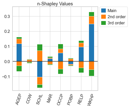
n_shapley_values.plot(feature_names = feature_names)

[9]:
<AxesSubplot:title={'center':'n-Shapley Values'}>
From the n-Shapley Values, we can obtain the 3-Shapley Values
[10]:
n_shapley_values.k_shapley_values(3).plot(feature_names = feature_names)
plt.show()
… Shapley Interaction Values (with the interventaional Shap Value function, these the SHAP interaction values from the shap package)
[11]:
n_shapley_values.k_shapley_values(2).plot(feature_names = feature_names)
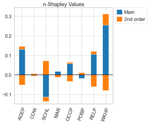
[11]:
<AxesSubplot:title={'center':'n-Shapley Values'}>
… and the usual Shapley Values
[12]:
n_shapley_values.k_shapley_values(1).plot(feature_names = feature_names)
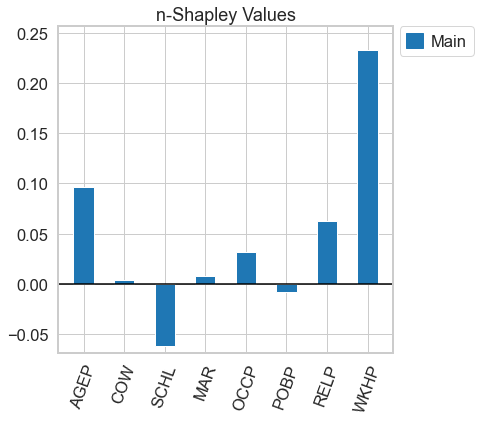
[12]:
<AxesSubplot:title={'center':'n-Shapley Values'}>
[13]:
import shap
shap.initjs()

[14]:
shap.force_plot(vfunc(X_test[0,:], []), n_shapley_values.shapley_values())
[14]:
Visualization omitted, Javascript library not loaded!
Have you run `initjs()` in this notebook? If this notebook was from another user you must also trust this notebook (File -> Trust notebook). If you are viewing this notebook on github the Javascript has been stripped for security. If you are using JupyterLab this error is because a JupyterLab extension has not yet been written.
Have you run `initjs()` in this notebook? If this notebook was from another user you must also trust this notebook (File -> Trust notebook). If you are viewing this notebook on github the Javascript has been stripped for security. If you are using JupyterLab this error is because a JupyterLab extension has not yet been written.
Let’s compare this to the Shapley Values from the shap package
[15]:
explainer = shap.KernelExplainer(gbtree.predict_proba, shap.kmeans(X_train, 25))

shap_values = explainer.shap_values(X_test[0, :])
[16]:
shap.force_plot(explainer.expected_value[0], shap_values[0])
[16]:
Visualization omitted, Javascript library not loaded!
Have you run `initjs()` in this notebook? If this notebook was from another user you must also trust this notebook (File -> Trust notebook). If you are viewing this notebook on github the Javascript has been stripped for security. If you are using JupyterLab this error is because a JupyterLab extension has not yet been written.
Have you run `initjs()` in this notebook? If this notebook was from another user you must also trust this notebook (File -> Trust notebook). If you are viewing this notebook on github the Javascript has been stripped for security. If you are using JupyterLab this error is because a JupyterLab extension has not yet been written.
Now, let us repeat this exercise with the the Shapley Taylor interaction index
[17]:
shapely_taylor = nshap.shapley_taylor(X_test[0, :], vfunc)
[18]:
shapely_taylor.save('shapley-taylor.json')
[19]:
shapely_taylor = nshap.load('shapley-taylor.json')
[20]:
# for n=d, both n-Shapley Values and the Shapley Taylor interaction index are equal to the Möbius transform, so we get the same picture as above
shapely_taylor.plot(feature_names = feature_names)
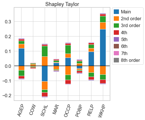
[20]:
<AxesSubplot:title={'center':'Shapley Taylor'}>
[21]:
nshap.allclose(n_shapley_values, shapely_taylor)
[21]:
True
[22]:
# more useful functions for the shapley taylor interaction index might come in the future. for now, we have to compute the index again for every order
k_shapely_taylor = nshap.shapley_taylor(X_test[0, :], vfunc, 3)
[23]:
# this plot, again, is almost the same as for 3-Shapley Values. A very close comparison of the two figures reveal, however, that they are not exactly the same
k_shapely_taylor.plot()
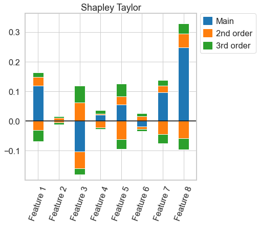
[23]:
<AxesSubplot:title={'center':'Shapley Taylor'}>
[24]:
nshap.allclose(n_shapley_values.k_shapley_values(3), k_shapely_taylor) # this confirms that the interaction indices are not exactly the same
[24]:
False
Now, the same exercise for Faith-Shap interaction index
[25]:
faith_shap = nshap.faith_shap(X_test[0, :], vfunc)
[26]:
faith_shap.save('faith-shap.json')
[27]:
faith_shap = nshap.load('faith-shap.json')
[28]:
# for n=d, both n-Shapley Values and the Faith-Shap index are equal to the Möbius transform, so we get the same picture as above
faith_shap.plot(feature_names = feature_names)

[28]:
<AxesSubplot:title={'center':'Faith-Shap'}>
[29]:
nshap.allclose(n_shapley_values, faith_shap)
[29]:
True
[30]:
# more useful functions for the Faith-Shap interaction index might come in the future. for now, we have to compute the index again for every order
k_faith_shap = nshap.faith_shap(X_test[0, :], vfunc, 3)
[31]:
# this plot, again, is almost the same as for 3-Shapley Values. A very close comparison of the two figures reveal, however, that they are not exactly the same
k_faith_shap.plot()
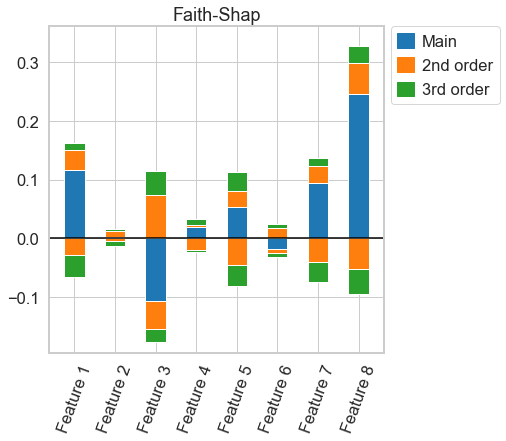
[31]:
<AxesSubplot:title={'center':'Faith-Shap'}>
[32]:
# again, the figure is very similar, but the interaction indices are not actually the same
nshap.allclose(n_shapley_values.k_shapley_values(3), k_faith_shap), nshap.allclose(k_shapely_taylor, k_faith_shap)
[32]:
(False, False)